transform in render detail
Coordinate System
Standard Basis
space空间是一个集合,如欧几里得空间是点集,是有序实数元组。
向量空间:欧几里得空间以向量的视角来看:欧几里得空间是起点到原点的向量集合。向量运算的结果是封闭closure的,满足一些性质。通常说的向量,就是欧几里得空间的元素。
广义向量空间:把非欧几里得空间的向量空间称为广义向量空间。
一个空间的基中,向量的个数称为维度。一个n维空间任何一组线性无关的向量,都是这个n维空间的一组基。n个非零正交向量一定是n维空间的基。
正交基:如果一个空间的一组基两两正交,则称这组基为一组正交基。标准正交基Orthogonal Basis:如果一个空间的一组正交基,模均为1,则称这组基是一组标准正交基。
从一维投影到高维投影,通过投影向量得到单位向量,就可以找出对应的一组正交基了。
格拉姆-施密特过程(Gram-Schmidt过程),就是求正交基的过程
空间的基与坐标系是一一对应的关系,在n维空间,如果给定一组基,任何一个向量都可以表示成这组基的线性组合,且表示方法唯一。其他坐标系与标准坐标系的转换,任意坐标系的互换,本质就是线性变换。
                        // pOrigin是原坐标系下的一个点
                        // xDir, yDir是单位向量值
                        // 构造旋转矩阵
                        const rmat = new Matrix3().identity();
                        rmat.elements[0 * 3 + 0] = xDir.x;
                        rmat.elements[1 * 3 + 0] = xDir.y;
                        rmat.elements[0 * 3 + 1] = yDir.x;
                        rmat.elements[1 * 3 + 1] = yDir.y;
                        rmat.invert();
                        const tmat = new Matrix3().identity();
                        tmat.makeTranslation(-pOrigin.x, -pOrigin.y);
                        // 坐标系
                        const matFrame = rmat.multiply(tmat);
                        // 这个可推广到三维坐标系的构建
Object Space
This is the coordinate system in which geometric primitives are defined. For example, spheres in pbrt are defined to be centered at the origin of their object space
World Space
While each primitive may have its own object space, all objects in the scene are placed in relation to a single world space. Each primitive has an object-to-world transformation that determines where it is located in world space. World space is the standard frame that all other spaces are defined in terms of.
Camera Space
A camera is placed in the scene at some world space point with a particular viewing direction and orientation. This camera defines a new coordinate system with its origin at the camera’s location. The \(Z\) axis of this coordinate system is mapped to the viewing direction, and the \(y\) axis is mapped to the up direction. This is a handy space for reasoning about which objects are potentially visible to the camera. For example, if an object’s camera space bounding box is entirely behind the \(Z=0\) plane (and the camera doesn’t have a field of view wider than 180 degrees), the object will not be visible to the camera.
Screen Space
Screen space is defined on the film plane. The camera projects objects in camera space onto the film plane; the parts inside the screen window are visible in the image that is generated. Depth values in screen space range from 0 to 1, corresponding to points at the near and far clipping planes, respectively. Note that, although this is called “screen” space, it is still a 3D coordinate system, since values are meaningful.
NDC(Normalized Device Coordinate) space
This is the coordinate system for the actual image being rendered. In \(x\) and \(y\), this space ranges from \((0,0)\) to \((1,1)\) , with \((0,0)\) being the upper-left corner of the image. Depth values are the same as in screen space, and a linear transformation converts from screen to NDC space.
Raster Space
This is almost the same as NDC space, except the \(x\) and \(y\) coordinates range from \((0,0)\) to \((resolution.x,resolution.y)\).
$$ \begin{bmatrix} x_{eye} \\ y_{eye} \\ z_{eye} \\ w_{eye} \end{bmatrix} = M_{view} \cdot M_{model} \cdot \begin{bmatrix} x_{obj} \\ y_{obj} \\ z_{obj} \\ w_{obj} \end{bmatrix} = M_{modelView} \cdot \begin{bmatrix} x_{obj} \\ y_{obj} \\ z_{obj} \\ w_{obj} \end{bmatrix} $$
$$ \begin{bmatrix} x_{clip} \\ y_{clip} \\ z_{clip} \\ w_{clip} \end{bmatrix} = M_{projection} \cdot \begin{bmatrix} x_{eye} \\ y_{eye} \\ z_{eye} \\ w_{eye} \end{bmatrix} = M_{projection} \cdot M_{view} \cdot M_{model} \cdot \begin{bmatrix} x_{obj} \\ y_{obj} \\ z_{obj} \\ w_{obj} \end{bmatrix} \label{refClipProject} $$
$$ \begin{bmatrix} x_{ndc} \\ y_{ndc} \\ z_{ndc} \end{bmatrix} = \begin{bmatrix} { x_{clip} \over w_{clip} } \\ { y_{clip} \over w_{clip} } \\ { z_{clip} \over w_{clip} } \end{bmatrix} \label{refNdcFromClip} $$
$$ \begin{bmatrix} x_{screen} \\ y_{screen} \\ z_{screen} \end{bmatrix} = \begin{bmatrix} { {width \over 2}x_{ndc} + (topX + {width \over 2}) } \\ { {height \over 2}y_{ndc} + (topY + {height \over 2}) } \\ { {{far - near} \over 2}z_{ndc} + {(far + near) \over 2}) } \end{bmatrix} \label{refScreenFromNdc} $$
[\ref{refScreenFromNdc}]对应的是glViewport(topX, topY, width, height)和glDepthRange(near, far)两个函数,取值范围也做了mapping映射
transform a normal vector from object to eye space
$$ \begin{bmatrix} nx_{eye} \\ ny_{eye} \\ nz_{eye} \\ nw_{eye} \\ \end{bmatrix} = (M_{modelView}^{-1})^{T} \begin{bmatrix} nx_{obj} \\ ny_{obj} \\ nz_{obj} \\ nw_{obj} \end{bmatrix} \label{refNormalTransform} $$
$$ \begin{bmatrix} n_{x} & n_{y} & n_{z} & n_{w} \end{bmatrix} \begin{bmatrix} x \\ y \\ z \\ w \end{bmatrix} = 0 \Rightarrow {n^T}v= 0 \label{refNormalTransform1} $$
现在来解释一下为什么[\ref{refNormalTransform}]是可行的?法线是决定光照效果的重要因素,光照是在eye space中处理的,法线也要引入eye space中来,法线与三角面片的关系如[\ref{refNormalTransform1}] 在其中间加入一个单位矩阵不影响结果,这样矩阵就变成如下,其法线与三角面片的关系也应该同时满足关系。
$$ \underbrace{ \begin{bmatrix} n_{x} & n_{y} & n_{z} & n_{w} \end{bmatrix} {M_{modelView}}^{-1} }_{normal transform} \times \underbrace{ M_{modelView} \begin{bmatrix} x \\ y \\ z \\ w \end{bmatrix} }_{vertex transofrm} = 0 $$
\({n^T}M^{-1}\)就是顶点法线从model space到eye space的变换
Conclusion
Transforming a normal vector from object space to eye space multiplying by inverse and transpose matrix would work if the transform matrix contains translation and rotation. However, if the transform has scaling, the normal vector must be re-normalized to make it unit length.
Since a rotation-only matrix is orthogonal (the inverse matrix and transpose matrix are same, so the original matrx and the inverse then transpose matrx are also identical), we can skip the process to invert and to transpose the matrix.
To optimize the performance of normal transformations, it would be better to define a separate matrix for the normal vectors, which is only containing the rotation parts from GL_MODELVIEW matrix (ignoring translation and scaling), and use this matrix to transform normal vectors from object space to eye space without computing inverse and transpose.
projection matrix
与normal matrix推理类似来推理投影矩阵的公式关系,glFrustum/glOrtho是OpenGL的NDC(Normalized Device Coordinate System)坐标系统,top是正y,bottom是负y,参数(left,right,bottom,top)就是(xmin, xmax, ymin, ymax)
perspective projection
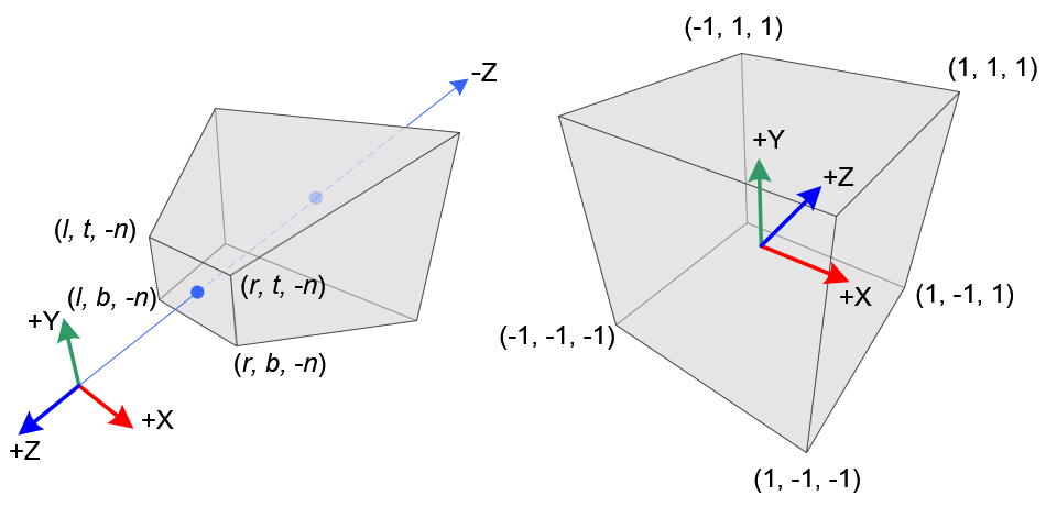
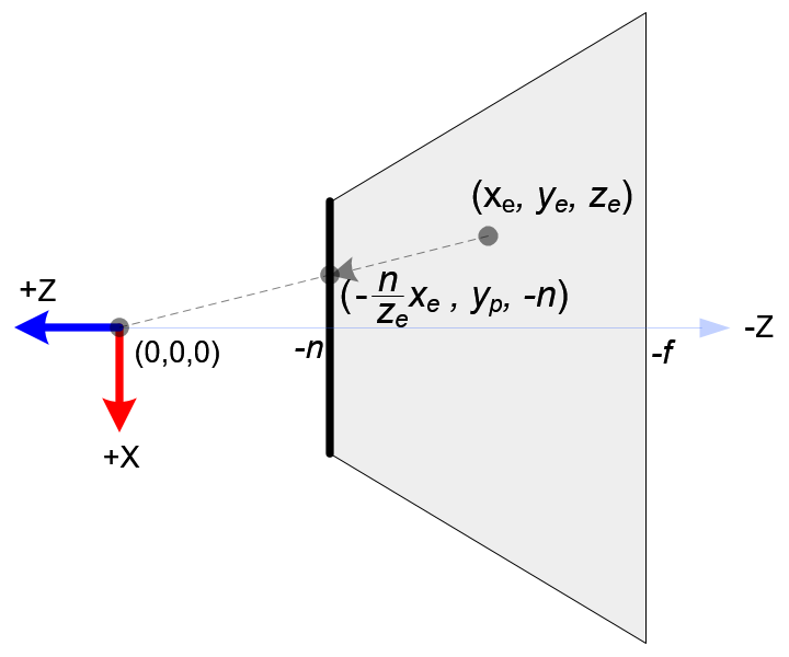
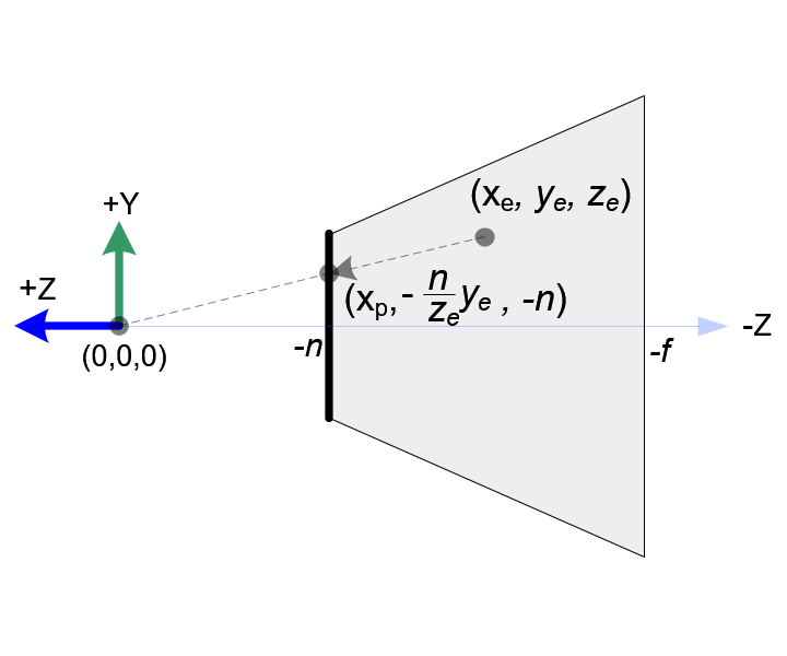
左边的图是projection到ndc的过程,中间的图是对frustum的顶视图截面,右边图是对frustum的侧面视图截面。
void glFrustum( GLdouble left, GLdouble right, GLdouble bottom, GLdouble top, GLdouble nearVal, GLdouble farVal);
利用三角形相似性,有如下公式
$$ {x_{proj} \over x_{eye}} = {{-near} \over {z_{eye}}} \Rightarrow x_{proj} = {{-near \cdot x_{eye}} \over {z_{eye}}} = {{near \cdot x_{eye}} \over {-z_{eye}}} \label{refPerspective1a} $$
$$ {y_{proj} \over y_{eye}} = {{-near} \over {z_{eye}}} \Rightarrow y_{proj} = {{-near \cdot y_{eye}} \over {z_{eye}}} = {{near \cdot y_{eye}} \over {-z_{eye}}} \label{refPerspective1b} $$
注意点\(x_{proj}\)和\(x_{proj}\)都依赖一个\(-z_{eye}\),由公式[\ref{refClipProject}]和[\ref{refNdcFromClip}]知道从eye space到clip space仍然是齐次坐标,在到NDC space过程中才除以\(w_{clip}\)的。 让\(w_{clip}=-z_{eye}\),则可以得出矩阵的应该满足如下模式[\ref{refPerspectiveX1}]
$$ \begin{bmatrix} x_{clip} \\ y_{clip} \\ z_{clip} \\ w_{clip} \end{bmatrix} = \begin{bmatrix} \cdot & \cdot & \cdot & \cdot \\ \cdot & \cdot & \cdot & \cdot \\ \cdot & \cdot & \cdot & \cdot \\ 0 & 0 & -1 & 0 \end{bmatrix} \cdot \begin{bmatrix} x_{eye} \\ y_{eye} \\ z_{eye} \\ w_{eye} \end{bmatrix} \label{refPerspectiveX1} $$
继续利用上面的三角形相似性,\(x_{proj}\)和\(y_{proj}\)到\(x_{ndc}\)和\(y_{ndc}\)满足的线性映射关系,因为由frustum的近平面到Cubic的front正面是一个平面与平面的变化,满足线性关系,\([left, right] \Rightarrow [-1,1] \)和\([bottom, top] \Rightarrow [-1,1] \) 对公式[\ref{refPerspective1}]代入\([x_{proj},x_{ndc}] = [right, 1]\)得到公式[\ref{refPerspective2}],就可以求出proje与ndc的关系[\ref{refPerspective3}]
$$ x_{ndc} = {{1 - (-1)} \over {right - left}} \cdot x_{proj} + \beta \label{refPerspective1} $$ $$ 1 = {{1 - (-1)} \over {right - left}} \cdot right + \beta \Rightarrow \beta = 1 - {{2right} \over {right - left}} = {{right - left - 2right} \over {right - left}} = -{{right + left} \over {right - left}} \label{refPerspective2} $$ $$ x_{ndc} = {2x_{proj} \over {right - left}} - {{right + left} \over {right - left}} \label{refPerspective3} $$
按照同样的逻辑可推理得到[\ref{refPerspective4}]
$$ y_{ndc} = {{1 - (-1)} \over {top - bottom}} \cdot y_{proj} + \beta $$ $$ 1 = {{1 - (-1)} \over {top - bottom}} \cdot top + \beta \Rightarrow \beta = 1 - {{2top} \over {top - bottom}} = {{top - bottom - 2top} \over {top - bottom}} = -{{top + bottom} \over {top - bottom}} $$ $$ y_{ndc} = {2x_{proj} \over {top - bottom}} - {{top + bottom} \over {top - bottom}} \label{refPerspective4} $$
现在可以把方程[\ref{refPerspective1a}]代入[\ref{refPerspective3}]求解
$$ x_{ndc} = {2x_{proj} \over {right - left}} - {{right + left} \over {right - left}} = {2{{near \cdot x_{eye}} \over {-z_{eye}}} \over {right - left}} - {{right + left} \over {right - left}} = (\underbrace{{{2near} \over {right - left}} \cdot x_{eye} + {{right + left} \over {right - left}} \cdot z_{eye}}_{x_{clip}})/-z_{eye} \label{refPerspective5} $$
现在可以把方程[\ref{refPerspective1b}]代入[\ref{refPerspective4}]求解
$$ y_{ndc} = {2y_{proj} \over {top - bottom}} - {{top + bottom} \over {top - bottom}} = {2{{near \cdot y_{eye}} \over {-z_{eye}}} \over {top - bottom}} - {{top + bottom} \over {top - bottom}} = (\underbrace{{{2near} \over {top - bottom}} \cdot y_{eye} + {{top + bottom} \over {top - bottom}} \cdot z_{eye}}_{y_{clip}})/-z_{eye} \label{refPerspective6} $$
矩阵[\ref{refPerspectiveX1}]现在代入[\ref{refPerspective5}]和[\ref{refPerspective6}]可以得到新的矩阵$$ \begin{bmatrix} x_{clip} \\ y_{clip} \\ z_{clip} \\ w_{clip} \end{bmatrix} = \begin{bmatrix} {2near \over {right - left}} & 0 & {{right + left} \over {right - left}} & 0 \\ 0 & {2near \over {top - bottom}} & {{top + bottom} \over {top - bottom}} & 0 \\ \cdot & \cdot & \cdot & \cdot \\ 0 & 0 & -1 & 0 \end{bmatrix} \cdot \begin{bmatrix} x_{eye} \\ y_{eye} \\ z_{eye} \\ w_{eye} \end{bmatrix} \label{refPerspectiveX2} $$
现在剩下第3行未知了,\(z_{ndc}\)不能像之前的\(x_{ndc},y_{ndc}\)那样求解,因为不满足线性关系,投影得到的\(z_{proj}\)只出现在近平面上,我们借用特殊情况下的值来推\(z_{ndc},z_{eye}\)之间的关系,可加设矩阵是如下格式
$$ \begin{bmatrix} x_{clip} \\ y_{clip} \\ z_{clip} \\ w_{clip} \end{bmatrix} = \begin{bmatrix} {2near \over {right - left}} & 0 & {{right + left} \over {right - left}} & 0 \\ 0 & {2near \over {top - bottom}} & {{top + bottom} \over {top - bottom}} & 0 \\ 0 & 0 & A & B \\ 0 & 0 & -1 & 0 \end{bmatrix} \cdot \begin{bmatrix} x_{eye} \\ y_{eye} \\ z_{eye} \\ w_{eye} \end{bmatrix} \label{refPerspectiveX3} $$
$$ \Rightarrow z_{ndc} = z_{clip} / w_{clip} = {{Az_{eye} + Bw_{eye}} \over {-z_{eye}}} \label{refPerspectiveX4} $$
$$ \Rightarrow z_{ndc} = {{Az_{eye} + B} \over {-z_{eye}}} \label{refPerspectiveX5} $$
$$ \begin{numcases}{} -1 = {{-A \cdot near + B} \over {near}} \\ 1 = {{-A \cdot far + B} \over {far}} \end{numcases} $$
$$ \begin{numcases}{} A = -{{far + near} \over {far - near}} \\ B = -{{2far \cdot near} \over {far - near}} \end{numcases} $$
矩阵相乘可得到公式[\ref{refPerspectiveX4}],对公式[\ref{refPerspectiveX4}],在eye space中一般设置为\(w_{eye}=1\),可得到简化的式子[\ref{refPerspectiveX5}],为求得系数\(A,B\)代入端点值 \([z_{eye},z_{ndc}], [-near,-1], [-far, 1]\)可推得系数\(A,B\),此时就可以得到最后的透视投影矩阵了[\ref{refPerspectiveX6}]
$$ \begin{bmatrix} x_{clip} \\ y_{clip} \\ z_{clip} \\ w_{clip} \end{bmatrix} = \begin{bmatrix} {2near \over {right - left}} & 0 & {{right + left} \over {right - left}} & 0 \\ 0 & {2near \over {top - bottom}} & {{top + bottom} \over {top - bottom}} & 0 \\ 0 & 0 & -{{far + near} \over {far - near}} & -{{2far \cdot near} \over {far - near}} \\ 0 & 0 & -1 & 0 \end{bmatrix} \cdot \begin{bmatrix} x_{eye} \\ y_{eye} \\ z_{eye} \\ w_{eye} \end{bmatrix} \label{refPerspectiveX6} $$
透视投影矩阵[\ref{refPerspectiveX6}]是一个通用的推理,对于特殊情况下还可以继续简化,就是对称frustum,此时有如下关系
$$ \begin{numcases}{} right + left = 0 \\ right - left = 2right_{width} \end{numcases} $$ $$ \begin{numcases}{} top + bottom = 0 \\ top - bottom = 2top_{heihgt} \end{numcases} $$
$$ m_{proj} = \begin{bmatrix} {near \over right} & 0 & 0 & 0 \\ 0 & {near \over top} & 0 & 0 \\ 0 & 0 & -{{far + near} \over {far - near}} & -{{2far \cdot near} \over {far - near}} \\ 0 & 0 & -1 & 0 \end{bmatrix} $$
orthorgraphics projection
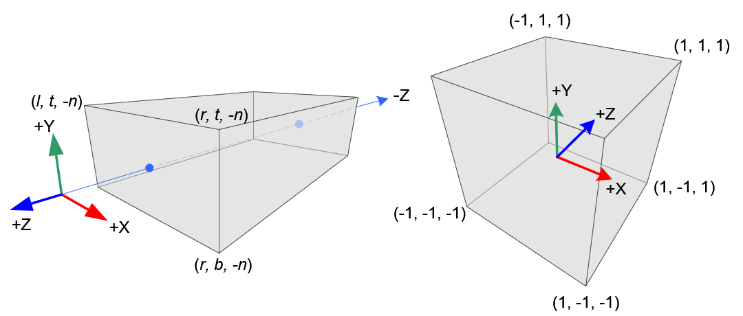
正交投影矩阵相比透视投影矩阵的推理要简化很多,因为三个轴向\(x_{eye},y_{eye},z_{eye}\)都满足线性关系,其线性映射推理与公式[\ref{refPerspective3}]和[\ref{refPerspective4}]是一样的逻辑, z轴代入的是\( [-f, 1]\), 注意near和far是传入的正值,推理时要加入负号
$$ x_{n} = {{1 - (-1)} \over {r - l}} \cdot x_{e} + \beta \Rightarrow 1 = {{1 - (-1)} \over {r - l}} \cdot r + \beta \Rightarrow \beta = 1 - {{2r} \over {r - l}} = -{{r + l} \over {r - l}} \Rightarrow x_{n} = {2 \over {r - l}} \cdot x_{e} - {{r + l} \over {r - l}} \label{refOrhtographicX1} $$
$$ y_{n} = {{1 - (-1)} \over {t - b}} \cdot y_{e} + \beta \Rightarrow 1 = {{1 - (-1)} \over {t - b}} \cdot t + \beta \Rightarrow \beta = 1 - {{2t} \over {t - b}} = -{{t + b} \over {t - b}} \Rightarrow y_{n} = {2 \over {t - b}} \cdot y_{e} - {{t + b} \over {t - b}} \label{refOrhtographicX2} $$
$$ z_{n} = {{1 - (-1)} \over {-f - (-n)}} \cdot z_{e} + \beta \Rightarrow 1 = {{1 - (-1)} \over {-f - (-n)}} \cdot (-f) + \beta \Rightarrow \beta = 1 - {{-2f} \over {-f - (-n)}} = -{{f + n} \over {f - n}} \Rightarrow z_{n} = {-2z_{e} \over {f - n}} - {{f + n} \over {f - n}} \label{refOrhtographicX3} $$
因为上面的映射关系是NDC与eye space下的关系,有\(x_{n} = {x_{clip} \over w_{clip}}\), 又因\(w_{e}=1\),可构造矩阵如下,让\(w_{clip}=1\)来满足上面的公式关系,就可以得到完整的正交投影矩阵[\ref{refOrhtographicX4}]
$$ \begin{bmatrix} x_{clip} \\ y_{clip} \\ z_{clip} \\ w_{clip} \end{bmatrix} = \begin{bmatrix} {2 \over {r - l}} & 0 & 0 & -{{r + l} \over {r - l}} \\ 0 & {2 \over {t - b}} & 0 & -{{t + b} \over {t - b}} \\ 0 & 0 & {{-2} \over {f - n}} & -{{f + n} \over {f - n}} \\ 0 & 0 & 0 & 1 \end{bmatrix} \cdot \begin{bmatrix} x_{e} \\ y_{e} \\ z_{e} \\ w_{e} \end{bmatrix} \label{refOrhtographicX4} $$
Depth and ViewZ
Perspective
threejs的src\renderers\shaders\ShaderChunk\packing.glsl.js中包含了两个函数,在examples\webgl_depth_texture.html中渲染深度,显示使用这个方法
                        float viewZToPerspectiveDepth( const in float viewZ, const in float near, const in float far ) {
                            return ( ( near + viewZ ) * far ) / ( ( far - near ) * viewZ );
                        }
                        float perspectiveDepthToViewZ( const in float invClipZ, const in float near, const in float far ) {
                            return ( near * far ) / ( ( far - near ) * invClipZ - far );
                        }
根据透视投影矩阵[\ref{refPerspectiveX6}]可得到关系,这里的\(view=eye\)有
$$ \begin{numcases}{} z_{clip} = -{{f + n} \over {f - n}} \times z_{view} + {-2fn \over {f - n}} \times {w_{view}} \\ w_{clip} = -z_{view} \end{numcases} $$
因为\(w_{view}=1\)和view(eye) space下的深度值 \(z = z_{view}, \)和[\ref{refNdcFromClip}] 所以有$$ z_{ndc} = {{z_{clip}} \over {w_{clip}}} = { {{-{f + n} \over {f - n}}z + {-2fn \over {f - n}}} \over -z} = {{ f + n + 2fn{1 \over z}} \over {f - n}} = {{ fz + nz + 2fn} \over {f - n}z } \label{refNdcEq} $$
$$ depth = {z_{ndc}{1 \over 2}} + {1 \over 2} \label{refDepthEq} $$
把 [\ref{refNdcEq}] 代入 [\ref{refDepthEq}] 可求解得到当前帧的深度值的表达式$$ depth = {{fz + nz + 2fn} \over {2(f - n)z}} + {{(f - n)z} \over {2(f - n)z}} = {{(n + z)f} \over {(f - n)z}} $$
知道帧的深度值可反求视图空间中的z坐标值, \(d = depth \)$$ d(f - n)z = (n + z)f \Rightarrow z(d(f - n) - f) = nf \Rightarrow z = { nf \over {d(f - n) -f}} $$
Orhtorgraphics
对正交矩阵的推理类型,根据式子[\ref{refOrhtographicX4}]可有
$$ \begin{numcases}{} z_{clip} = {-2 \over {f - n}} \times z_{view} - {{f + n} \over {f - n}} \times {w_{view}} \\ w_{clip} = w_{view} \end{numcases} $$
因为\(w_{view}=1\)和view(eye) space下的深度值 \(z = z_{view}, \)和[\ref{refNdcFromClip}] 所以有$$ z_{ndc} = {{z_{clip}} \over {w_{clip}}} = { {{-2} \over {f - n}}z - {{f + n} \over {f - n}} \over 1} = -{{ 2z + f + n} \over {f - n}} \label{refNdcEqOrth1} $$
把 [\ref{refNdcEqOrth1}] 代入 [\ref{refDepthEq}] 可求解得到当前帧的深度值的表达式
$$ depth = -{{2z + f + n} \over {2(f - n)}} + {{(f - n)} \over {2(f - n)}} = {{-2z - f - n + f - n} \over {2(f - n)}} = {{(z + n)} \over {n - f}} $$
知道帧的深度值可反求视图空间中的z坐标值, \(d = depth \)$$ d(n - f) = (z + n) \Rightarrow d(n - f) - n = z \Rightarrow z = {{d(n - f) - n}} $$
其glsl的代码也可以得到
                        // NOTE: viewZ/eyeZ is < 0 when in front of the camera per OpenGL conventions

                        float viewZToOrthographicDepth( const in float viewZ, const in float near, const in float far ) {
                            return ( viewZ + near ) / ( near - far );
                        }
                        float orthographicDepthToViewZ( const in float linearClipZ, const in float near, const in float far ) {
                            return linearClipZ * ( near - far ) - near;
                        }
screen positin to view position
                        vec3 getViewPosition(const in vec2 screenPosition, const in float depth, const in float viewZ) {
                            // clip = A * viewZ + B
                            float clipW = cameraProjectionMatrix[2][3] * viewZ + cameraProjectionMatrix[3][3];
                            // ndc to clip
                            vec4 clipPosition = vec4((vec3(screenPosition, depth) - 0.5) * 2.0, 1.0);
                            clipPosition *= clipW;
                            // clip = projection * view => view => projection'-1 * clip
                            return (cameraInverseProjectionMatrix * clipPosition).xyz;
                        }
参考
符合含义
\(n\) camera near
\(f\) camera far